Figure A6. Scatter plot of the budget residuals (i.e. altimetry
4.8 (152) · € 33.00 · En Stock
Download scientific diagram | Figure A6. Scatter plot of the budget residuals (i.e. altimetry minus sum of components) against the area of each domain for δ-MAPS (red) and SOM (blue). Stars and circles indicate domains in which the sea-level budget is open and closed, respectively. As the domain area increases, the residuals converge towards 0. All the SOM residuals are within ±1 mm yr −1 , as are 74.2 % of the δ-MAPS domains. from publication: Regionalizing the sea-level budget with machine learning techniques | Attribution of sea-level change to its different drivers is typically done using a sea-level budget approach. While the global mean sea-level budget is considered closed, closing the budget on a finer spatial scale is more complicated due to, for instance, limitations in our | Budget, Regionalism and Machine Learning | ResearchGate, the professional network for scientists.
Fluids, Free Full-Text
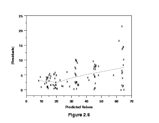
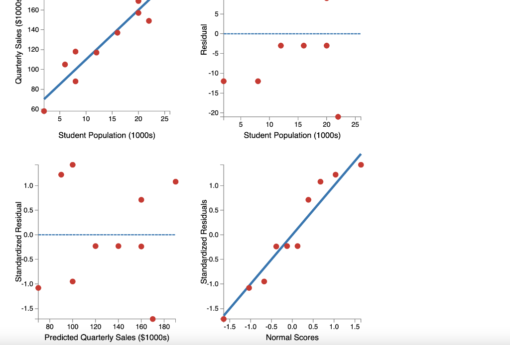
5.2.4. Are the model residuals well-behaved?
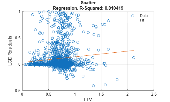
Scatter plot of predicted and observed LGDs - MATLAB

Stirring of Interior Potential Vorticity Gradients as a Formation

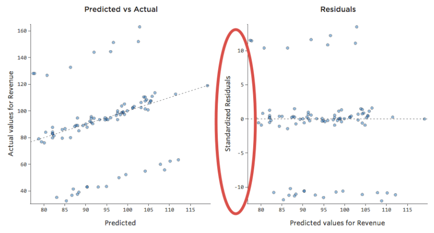
A, Scatter plot of observed by predicted values and, B

Wind–Wave Interaction for Strong Winds in: Journal of Physical

Remote Sensing, Free Full-Text

Wind speed and mesoscale features drive net autotrophy in the

Bayesian parameter estimation in glacier mass-balance modelling
Remote Sensing, Free Full-Text
Solved Diagnostic Residual Plots - Armand's Pizza Conceptual

Wind speed and mesoscale features drive net autotrophy in the

Implementation of a 1‐D Thermodynamic Model for Simulating the
Interpreting Residual Plots to Improve Your Regression